Visualizations, Buttons, sliders, filters, n-D plots, plots vs graphs
In previous chapter, We created Finance datasets samples.
In this section, we will again look into few examples.
These examples show case how to use, sliders, inputs, select boxes to dynamically change data and see data changes.
Since this documentation is a static web page, at present, these example will NOT update data.
In future, I will deploy my Pluto notebooks at Pluto server and update these sections to see live data. However, these code samples works well in local or remote Pluto server environment.
TODO: host Pluto notebook here.
Would, Could, Should, What if scenarios
Below sliders, help update/filter data.
For example, User can select LEDGER TYPE, OPERATINGREGION, FISCALYEAR, LOCATIONS/REGIONS, ACCOUNT/LOCATION ROLL UP to change data dynamically.
sample PlutoUI sliders/input image
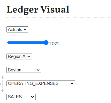
additionally, Sliders are use to update data without change actual data for comparison.
what if
- Region A is merged with Region B
- Employee resume work from office, how much Travel amounts % will increase.
- % of Office supply expenses given to Employee as home office setup
- would Region A, Cash Flow Investment have returned 7% ROI
- would Region B received Government/investor funding
- could have increased IT operating expenses by 5%
- could have reduced HR temp staff
- should have paid vendor invoiced on time to recive rebate
- should have applied loan to increase production
- should have retired a particular Asset
Income, Cash-Flow & Balance sheet statements
below is sample Finance Ledger Data with slicers, inputs
julia> using DataFrames, Plots, Datesjulia> # create default binding values/params using PlutoUIjulia> ## WARNING ## These bind variable will throw in error in documentation ## however, these runs fine on Pluto notebooks and provide a slider to change values dynamically # @bind ld Select(["Actuals", "Budget"]) # @bind rg Select(["Region A", "Region B", "Region C"]) # @bind yr Slider(2020:1:2021, default=2020, show_value=true) # @bind qtr Slider(1:1:4, default=1, show_value=true) # @bind ld_p Select(["Actuals", "Budget"]) # @bind yr_p Slider(2020:1:2021, default=2021, show_value=true) # @bind rg_p Select(["Region A", "Region B", "Region C"]) # @bind ldescr Select(unique(location.DESCR)) # @bind adescr Select(unique(accounts.CLASSIFICATION)) # @bind ddescr Select(unique(dept.CLASSIFICATION)) # create dummy data accounts = DataFrame(AS_OF_DATE=Date("1900-01-01", dateformat"y-m-d"), ID = 11000:1000:45000, CLASSIFICATION=repeat([ "OPERATING_EXPENSES","NON-OPERATING_EXPENSES", "ASSETS","LIABILITIES", "NET_WORTH","STATISTICS","REVENUE" ], inner=5), CATEGORY=[ "Travel","Payroll","non-Payroll","Allowance","Cash", "Facility","Supply","Services","Investment","Misc.", "Depreciation","Gain","Service","Retired","Fault.", "Receipt","Accrual","Return","Credit","ROI", "Cash","Funds","Invest","Transfer","Roll-over", "FTE","Members","Non_Members","Temp","Contractors", "Sales","Merchant","Service","Consulting","Subscriptions" ], STATUS="A", DESCR=repeat([ "operating expenses","non-operating expenses", "assets","liability","net-worth","stats","revenue" ], inner=5), ACCOUNT_TYPE=repeat([ "E","E","A","L","N","S","R" ],inner=5));julia> dept = DataFrame(AS_OF_DATE=Date("2000-01-01", dateformat"y-m-d"), ID = 1100:100:1500, CLASSIFICATION=[ "SALES","HR", "IT","BUSINESS","OTHERS" ], CATEGORY=[ "sales","human_resource","IT_Staff","business","others" ], STATUS="A", DESCR=[ "Sales & Marketing","Human Resource","Infomration Technology","Business leaders","other temp" ], DEPT_TYPE=[ "S","H","I","B","O"]);julia> location = DataFrame(AS_OF_DATE=Date("2000-01-01", dateformat"y-m-d"), ID = 11:1:22, CLASSIFICATION=repeat([ "Region A","Region B", "Region C"], inner=4), CATEGORY=repeat([ "Region A","Region B", "Region C"], inner=4), STATUS="A", DESCR=[ "Boston","New York","Philadelphia","Cleveland","Richmond", "Atlanta","Chicago","St. Louis","Minneapolis","Kansas City", "Dallas","San Francisco"], LOCA_TYPE="Physical");julia> ledger = DataFrame( LEDGER = String[], FISCAL_YEAR = Int[], PERIOD = Int[], ORGID = String[], OPER_UNIT = String[], ACCOUNT = Int[], DEPT = Int[], LOCATION = Int[], POSTED_TOTAL = Float64[] );julia> # create 2020 Period 1-12 Actuals Ledger l = "Actuals";julia> fy = 2020;julia> for p = 1:12 for i = 1:10^5 push!(ledger, (l, fy, p, "ABC Inc.", rand(location.CATEGORY), rand(accounts.ID), rand(dept.ID), rand(location.ID), rand()*10^8)) end endjulia> # create 2021 Period 1-4 Actuals Ledger l = "Actuals";julia> fy = 2021;julia> for p = 1:4 for i = 1:10^5 push!(ledger, (l, fy, p, "ABC Inc.", rand(location.CATEGORY), rand(accounts.ID), rand(dept.ID), rand(location.ID), rand()*10^8)) end endjulia> # create 2021 Period 1-4 Budget Ledger l = "Budget";julia> fy = 2021;julia> for p = 1:12 for i = 1:10^5 push!(ledger, (l, fy, p, "ABC Inc.", rand(location.CATEGORY), rand(accounts.ID), rand(dept.ID), rand(location.ID), rand()*10^8)) end endjulia> ledger[:,:]2800000×9 DataFrame Row │ LEDGER FISCAL_YEAR PERIOD ORGID OPER_UNIT ACCOUNT DEPT ⋯ │ String Int64 Int64 String String Int64 Int64 ⋯ ─────────┼────────────────────────────────────────────────────────────────────── 1 │ Actuals 2020 1 ABC Inc. Region A 39000 1500 ⋯ 2 │ Actuals 2020 1 ABC Inc. Region A 16000 1100 3 │ Actuals 2020 1 ABC Inc. Region C 30000 1400 4 │ Actuals 2020 1 ABC Inc. Region A 12000 1100 5 │ Actuals 2020 1 ABC Inc. Region B 13000 1500 ⋯ 6 │ Actuals 2020 1 ABC Inc. Region C 17000 1500 7 │ Actuals 2020 1 ABC Inc. Region A 44000 1100 8 │ Actuals 2020 1 ABC Inc. Region A 36000 1300 ⋮ │ ⋮ ⋮ ⋮ ⋮ ⋮ ⋮ ⋮ ⋱ 2799994 │ Budget 2021 12 ABC Inc. Region C 43000 1200 ⋯ 2799995 │ Budget 2021 12 ABC Inc. Region B 38000 1400 2799996 │ Budget 2021 12 ABC Inc. Region A 14000 1300 2799997 │ Budget 2021 12 ABC Inc. Region A 16000 1200 2799998 │ Budget 2021 12 ABC Inc. Region C 26000 1400 ⋯ 2799999 │ Budget 2021 12 ABC Inc. Region C 18000 1300 2800000 │ Budget 2021 12 ABC Inc. Region B 39000 1300 2 columns and 2799985 rows omittedjulia> # Create Finance Statements ld = "Actuals""Actuals"julia> rg = "Region B""Region B"julia> yr = 20202020julia> qtr = 11julia> ld_p = "Actuals""Actuals"julia> rg_p = "Region B""Region B"julia> yr_p = 20202020julia> qtr_p = 11julia> ldescr = unique(location.DESCR)12-element Vector{String}: "Boston" "New York" "Philadelphia" "Cleveland" "Richmond" "Atlanta" "Chicago" "St. Louis" "Minneapolis" "Kansas City" "Dallas" "San Francisco"julia> adescr = unique(accounts.CLASSIFICATION)7-element Vector{String}: "OPERATING_EXPENSES" "NON-OPERATING_EXPENSES" "ASSETS" "LIABILITIES" "NET_WORTH" "STATISTICS" "REVENUE"julia> ddescr = unique(dept.CLASSIFICATION)5-element Vector{String}: "SALES" "HR" "IT" "BUSINESS" "OTHERS"julia> ######################## ##### BALANCE SHEET #### ######################## # rename dimensions columns for innerjoin df_accounts = rename(accounts, :ID => :ACCOUNTS_ID, :CLASSIFICATION => :ACCOUNTS_CLASSIFICATION, :CATEGORY => :ACCOUNTS_CATEGORY, :DESCR => :ACCOUNTS_DESCR);julia> df_dept = rename(dept, :ID => :DEPT_ID, :CLASSIFICATION => :DEPT_CLASSIFICATION, :CATEGORY => :DEPT_CATEGORY, :DESCR => :DEPT_DESCR);julia> df_location = rename(location, :ID => :LOCATION_ID, :CLASSIFICATION => :LOCATION_CLASSIFICATION, :CATEGORY => :LOCATION_CATEGORY, :DESCR => :LOCATION_DESCR);julia> # create a function which converts accounting period to Quarter function periodToQtr(x) if x ∈ 1:3 return 1 elseif x ∈ 4:6 return 2 elseif x ∈ 7:9 return 3 else return 4 end endperiodToQtr (generic function with 1 method)julia> ############################################################## # create a new dataframe to join all chartfields with ledger # ############################################################## df_ledger = innerjoin( innerjoin( innerjoin(ledger, df_accounts, on = [:ACCOUNT => :ACCOUNTS_ID], makeunique=true), df_dept, on = [:DEPT => :DEPT_ID], makeunique=true), df_location, on = [:LOCATION => :LOCATION_ID], makeunique=true);julia> transform!(df_ledger, :PERIOD => ByRow(periodToQtr) => :QTR);julia> function numToCurrency(x) return string("USD ",round(x/10^6; digits = 2), "m") endnumToCurrency (generic function with 1 method)julia> gdf = groupby(df_ledger, [:LEDGER, :FISCAL_YEAR, :QTR, :OPER_UNIT, :ACCOUNTS_CLASSIFICATION, :DEPT_CLASSIFICATION, # :LOCATION_CLASSIFICATION, :LOCATION_DESCR]);julia> gdf_plot = combine(gdf, :POSTED_TOTAL => sum => :TOTAL);julia> select(gdf_plot[( (gdf_plot.FISCAL_YEAR .== yr) .& (gdf_plot.QTR .== qtr) .& (gdf_plot.LEDGER .== ld) .& (gdf_plot.OPER_UNIT .== rg) ),:], :FISCAL_YEAR => :FY, :QTR => :Qtr, :OPER_UNIT => :Org, :ACCOUNTS_CLASSIFICATION => :Accounts, :DEPT_CLASSIFICATION => :Dept, # :LOCATION_CLASSIFICATION => :Region, :LOCATION_DESCR => :Loc, :TOTAL => ByRow(numToCurrency) => :TOTAL)420×7 DataFrame Row │ FY Qtr Org Accounts Dept Loc ⋯ │ Int64 Int64 String String String String ⋯ ─────┼────────────────────────────────────────────────────────────────────────── 1 │ 2020 1 Region B OPERATING_EXPENSES OTHERS New York ⋯ 2 │ 2020 1 Region B LIABILITIES OTHERS Cleveland 3 │ 2020 1 Region B NET_WORTH OTHERS Chicago 4 │ 2020 1 Region B NON-OPERATING_EXPENSES BUSINESS Kansas City 5 │ 2020 1 Region B NET_WORTH IT Richmond ⋯ 6 │ 2020 1 Region B LIABILITIES OTHERS Chicago 7 │ 2020 1 Region B ASSETS IT New York 8 │ 2020 1 Region B OPERATING_EXPENSES SALES Boston ⋮ │ ⋮ ⋮ ⋮ ⋮ ⋮ ⋮ ⋱ 414 │ 2020 1 Region B OPERATING_EXPENSES OTHERS Kansas City ⋯ 415 │ 2020 1 Region B LIABILITIES HR Dallas 416 │ 2020 1 Region B REVENUE HR Minneapolis 417 │ 2020 1 Region B ASSETS OTHERS Philadelphia 418 │ 2020 1 Region B LIABILITIES BUSINESS Boston ⋯ 419 │ 2020 1 Region B STATISTICS HR Chicago 420 │ 2020 1 Region B ASSETS OTHERS Minneapolis 1 column and 405 rows omittedjulia> ######################## ### Income Statement ### ######################## select(gdf_plot[( (gdf_plot.FISCAL_YEAR .== yr) .& (gdf_plot.QTR .== qtr) .& (gdf_plot.LEDGER .== ld) .& (gdf_plot.OPER_UNIT .== rg) .& (in.(gdf_plot.ACCOUNTS_CLASSIFICATION, Ref(["ASSETS", "LIABILITIES", "REVENUE","NET_WORTH"]))) ),:], :FISCAL_YEAR => :FY, :QTR => :Qtr, :OPER_UNIT => :Org, :ACCOUNTS_CLASSIFICATION => :Accounts, # :DEPT_CLASSIFICATION => :Dept, # :LOCATION_CLASSIFICATION => :Region, # :LOCATION_DESCR => :Loc, :TOTAL => ByRow(numToCurrency) => :TOTAL)240×5 DataFrame Row │ FY Qtr Org Accounts TOTAL │ Int64 Int64 String String String ─────┼──────────────────────────────────────────────────── 1 │ 2020 1 Region B LIABILITIES USD 12768.44m 2 │ 2020 1 Region B NET_WORTH USD 13499.34m 3 │ 2020 1 Region B NET_WORTH USD 12099.88m 4 │ 2020 1 Region B LIABILITIES USD 11484.86m 5 │ 2020 1 Region B ASSETS USD 12274.09m 6 │ 2020 1 Region B LIABILITIES USD 11617.84m 7 │ 2020 1 Region B NET_WORTH USD 11411.07m 8 │ 2020 1 Region B ASSETS USD 12781.2m ⋮ │ ⋮ ⋮ ⋮ ⋮ ⋮ 234 │ 2020 1 Region B NET_WORTH USD 11496.22m 235 │ 2020 1 Region B LIABILITIES USD 11857.41m 236 │ 2020 1 Region B LIABILITIES USD 12326.16m 237 │ 2020 1 Region B REVENUE USD 10935.97m 238 │ 2020 1 Region B ASSETS USD 10607.67m 239 │ 2020 1 Region B LIABILITIES USD 11059.42m 240 │ 2020 1 Region B ASSETS USD 12439.36m 225 rows omittedjulia> ######################## ##### CASH FLOW ######## ######################## select(gdf_plot[( (gdf_plot.FISCAL_YEAR .== yr) .& (gdf_plot.QTR .== qtr) .& (gdf_plot.LEDGER .== ld) .& (gdf_plot.OPER_UNIT .== rg) .& (in.(gdf_plot.ACCOUNTS_CLASSIFICATION, Ref(["NON-OPERATING_EXPENSES","OPERATING_EXPENSES" ]))) ),:], :FISCAL_YEAR => :FY, :QTR => :Qtr, :OPER_UNIT => :Org, :ACCOUNTS_CLASSIFICATION => :Accounts, # :DEPT_CLASSIFICATION => :Dept, # :LOCATION_CLASSIFICATION => :Region, # :LOCATION_DESCR => :Loc, :TOTAL => ByRow(numToCurrency) => :TOTAL)120×5 DataFrame Row │ FY Qtr Org Accounts TOTAL │ Int64 Int64 String String String ─────┼─────────────────────────────────────────────────────────────── 1 │ 2020 1 Region B OPERATING_EXPENSES USD 12555.49m 2 │ 2020 1 Region B NON-OPERATING_EXPENSES USD 11605.1m 3 │ 2020 1 Region B OPERATING_EXPENSES USD 11293.62m 4 │ 2020 1 Region B OPERATING_EXPENSES USD 11044.87m 5 │ 2020 1 Region B OPERATING_EXPENSES USD 11324.14m 6 │ 2020 1 Region B NON-OPERATING_EXPENSES USD 10966.59m 7 │ 2020 1 Region B NON-OPERATING_EXPENSES USD 12681.28m 8 │ 2020 1 Region B NON-OPERATING_EXPENSES USD 11180.16m ⋮ │ ⋮ ⋮ ⋮ ⋮ ⋮ 114 │ 2020 1 Region B NON-OPERATING_EXPENSES USD 12131.92m 115 │ 2020 1 Region B OPERATING_EXPENSES USD 11081.52m 116 │ 2020 1 Region B NON-OPERATING_EXPENSES USD 13179.55m 117 │ 2020 1 Region B OPERATING_EXPENSES USD 10241.69m 118 │ 2020 1 Region B OPERATING_EXPENSES USD 12451.05m 119 │ 2020 1 Region B NON-OPERATING_EXPENSES USD 12485.48m 120 │ 2020 1 Region B OPERATING_EXPENSES USD 11771.16m 105 rows omittedjulia> ######################## ##### Ledger Visual #### ######################## plot_data = gdf_plot[( (gdf_plot.FISCAL_YEAR .== yr_p) .& (gdf_plot.LEDGER .== ld_p) .& (gdf_plot.OPER_UNIT .== rg_p) .& (gdf_plot.LOCATION_DESCR .== ldescr) .& (gdf_plot.DEPT_CLASSIFICATION .== ddescr) .& (gdf_plot.ACCOUNTS_CLASSIFICATION .== adescr)) , :];ERROR: DimensionMismatch: arrays could not be broadcast to a common size; got a dimension with lengths 12600 and 12julia> # @df plot_data scatter(:QTR, :TOTAL/10^8, title = "Finance Ledger Data", xlabel="Quarter", ylabel="Total (in USD million)", label="$ld_p Total by $yr_p for $rg_p") @df plot_data plot(:QTR, :TOTAL/10^8, title = "Finance Ledger Data", xlabel="Quarter", ylabel="Total (in USD million)", label=[ "$ld_p by $yr_p for $rg_p $ldescr $adescr $ddescr" ], lw=3)ERROR: LoadError: UndefVarError: `@df` not defined in expression starting at REPL[41]:1julia> ################################# ## Actual vs Budget Comparison ## ################################# plot_data_a = gdf_plot[( (gdf_plot.FISCAL_YEAR .== yr_p) .& (gdf_plot.LEDGER .== "Actuals") .& (gdf_plot.OPER_UNIT .== rg_p) .& (gdf_plot.LOCATION_DESCR .== ldescr) .& (gdf_plot.DEPT_CLASSIFICATION .== ddescr) .& (gdf_plot.ACCOUNTS_CLASSIFICATION .== adescr)) , :];ERROR: DimensionMismatch: arrays could not be broadcast to a common size; got a dimension with lengths 12600 and 12julia> # @df plot_data scatter(:QTR, :TOTAL/10^8, title = "Finance Ledger Data", xlabel="Quarter", ylabel="Total (in USD million)", label="$ld_p Total by $yr_p for $rg_p") plot_data_b = gdf_plot[( (gdf_plot.FISCAL_YEAR .== yr_p) .& (gdf_plot.LEDGER .== "Budget") .& (gdf_plot.OPER_UNIT .== rg_p) .& (gdf_plot.LOCATION_DESCR .== ldescr) .& (gdf_plot.DEPT_CLASSIFICATION .== ddescr) .& (gdf_plot.ACCOUNTS_CLASSIFICATION .== adescr)) , :];ERROR: DimensionMismatch: arrays could not be broadcast to a common size; got a dimension with lengths 12600 and 12julia> # @df plot_data scatter(:QTR, :TOTAL/10^8, title = "Finance Ledger Data", xlabel="Quarter", ylabel="Total (in USD million)", label="$ld_p Total by $yr_p for $rg_p") @df plot_data_a plot(:QTR, :TOTAL/10^8, title = "Finance Ledger Data", xlabel="Quarter", ylabel="Total (in USD million)", label=[ "Actuals by $yr_p for $rg_p $ldescr $adescr $ddescr" ], lw=3)ERROR: LoadError: UndefVarError: `@df` not defined in expression starting at REPL[44]:1julia> @df plot_data_b plot!(:QTR, :TOTAL/10^8, title = "Finance Ledger Data", xlabel="Quarter", ylabel="Total (in USD million)", label=[ "Budget by $yr_p for $rg_p $ldescr $adescr $ddescr" ], lw=3)ERROR: LoadError: UndefVarError: `@df` not defined in expression starting at REPL[45]:1
Dynamic roll ups
Invoices by Diversity Vendor groups
Vendor Ranking
Product Ranking
Cost per Invoice
Operating Expenses trend
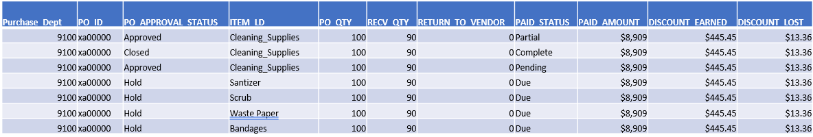
Supply chain Inventory Dashboard
below is an example dashboard (image) built in Pluto
This dashboard uses OnlineStats.jl for "real-time" udpates